KV Cache Optimization via Tensor Product Attention

digitado ⋅ 8 de dezembro de 2025

Table of Contents

KV Cache Optimization via Tensor Product Attention

In the first two lessons of this series, we explored how modern attention mechanisms like Grouped Query Attention (GQA) and Multi-Head Latent Attention (MLA) can significantly reduce the memory footprint of key-value (KV) caches during inference. GQA introduced a clever way to share keys and values across query groups, striking a balance between expressiveness and efficiency. MLA took this further by learning a compact latent space for attention heads, enabling more scalable inference without sacrificing model quality.

Now, in this third installment, we dive into Tensor Product Attention (TPA) — a novel approach that reimagines the very structure of attention representations. TPA leverages tensor decompositions to factorize queries, keys, and values into low-rank contextual components, enabling a highly compact and expressive representation. This not only slashes KV cache size but also integrates seamlessly with Rotary Positional Embeddings (RoPE), preserving positional awareness.

In this tutorial, we will unpack the mechanics of TPA, its role in KV cache optimization, and how it paves the way for scalable, high-performance LLM inference.

This lesson is the last of a 3-part series on LLM Inference Optimization — KV Cache:

Introduction to KV Cache Optimization Using Grouped Query Attention
KV Cache Optimization via Multi-Head Latent Attention
KV Cache Optimization via Tensor Product Attention (this tutorial)

To learn how to optimize KV Cache using Tensor Product Attention, just keep reading.

Looking for the source code to this post?

Jump Right To The Downloads Section

Challenges with Grouped Query and Multi-Head Latent Attention

Before diving into Tensor Product Attention (TPA), it’s important to understand the limitations of existing KV cache optimization strategies — particularly Grouped Query Attention (GQA) and Multi-Head Latent Attention (MLA) — and why they fall short in scaling inference efficiently.

Multi-Head Attention (MHA)

Standard Multi-Head Attention computes attention independently across multiple heads, each with its own set of query, key, and value projections:

$text{Attention}(Q, K, V) = text{softmax}left(dfrac{QK^top}{sqrt{d_k}}right)V$

Each head $h$ uses its own projections $W^K_h, W^V_h$ , resulting in a KV cache size that scales linearly with the number of heads and sequence length. While expressive, this design incurs significant memory overhead during inference.

Grouped Query Attention (GQA)

GQA reduces KV cache size by sharing keys and values across groups of query heads. If $H$ is the number of query heads and $G$ is the number of key-value groups, then each group shares:

$K_g = W^K_g X, quad V_g = W^V_g X quad text{for } g = 1, dots, G$

This reduces cache size from $H times L$ to $G times L$ , where $L$ is the sequence length. However, GQA sacrifices flexibility — fewer key-value groups mean less granularity in attention — and often requires architectural changes to balance performance and efficiency.

Multi-Head Latent Attention (MLA)

MLA, introduced in DeepSeek-V2, compresses KV representations by projecting them into a shared latent space:

$K' = W^K_{text{latent}} K, quad V' = W^V_{text{latent}} V$

This latent compression reduces memory usage, but integrating Rotary Positional Embeddings (RoPE) becomes problematic. RoPE typically operates per-head, and MLA’s shared latent space necessitates additional position-encoded parameters per head, complicating implementation and increasing overhead.

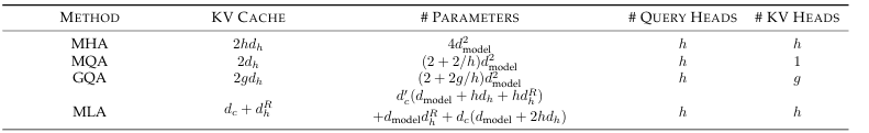
Table 1 summarizes the KV cache size for the above attention methods as a function of sequence length, model hidden dimension, and number of heads.

**Table 1:** Comparison of different attention mechanisms such as MHA, GQA, MLA, etc. (source: Zhang et al., 2025).

Tensor Product Attention (TPA)

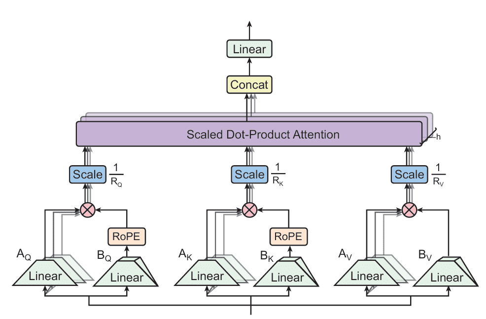
Tensor Product Attention (TPA) is a novel attention mechanism designed to address the memory bottlenecks of traditional multi-head attention (MHA) during inference. Unlike prior methods that statically compress weights or share KV states across heads, TPA dynamically factorizes the activations — the queries, keys, and values — into low-rank components. This enables compact, expressive representations that drastically reduce KV cache size while preserving model quality (Figure 1).

**Figure 1:** Illustration of Tensor Product Attention (source: Zhang et al., 2025).

TPA: Tensor Decomposition of Q, K, V

TPA replaces each head’s query, key, and value vectors with a sum of tensor products of latent factors derived from the token’s hidden state $(x_t)$ . Specifically, for each token $(t)$ :

$Q_t = dfrac{1}{R_Q} displaystylesum_{r=1}^{R_Q} A_Q^{(r)}(x_t) otimes B_Q^{(r)}(x_t) in mathbb{R}^{H times d_h}$

$K_t = dfrac{1}{R_K} displaystylesum_{r=1}^{R_K} A_K^{(r)}(x_t) otimes B_K^{(r)}(x_t) in mathbb{R}^{H times d_h}$

$V_t = dfrac{1}{R_V} displaystylesum_{r=1}^{R_V} A_V^{(r)}(x_t) otimes B_V^{(r)}(x_t) in mathbb{R}^{H times d_h}$

Here:

$R_Q, R_K, R_V$ are the decomposition ranks
Each factor map $A^{(r)}(cdot), B^{(r)}(cdot)$ is a learned function of $x_t$
The outer product $otimes$ produces a rank-1 matrix per factor

This formulation allows each token’s KV state to be stored as a compact set of low-rank factors, reducing cache size to $mathcal{O}(T cdot R cdot (H + d_h))$ , where $R = max(R_Q, R_K, R_V)$ .

Latent Factor Maps and Efficient Implementation

Each factor $A^{(r)}(cdot), B^{(r)}(cdot)$ is computed via linear projections from the token embedding:

$A_Q^{(r)}(x_t) = W^a_Q x_t in mathbb{R}^H, quad B_Q^{(r)}(x_t) = W^b_Q x_t in mathbb{R}^{d_h}$

To simplify implementation, the rank index is merged into a single output dimension:

$A_Q(x_t) in mathbb{R}^{R_Q times H}, quad B_Q(x_t) in mathbb{R}^{R_Q times d_h}$

The final query slice is computed as:

$Q_t = dfrac{1}{R_Q} A_Q(x_t)^top B_Q(x_t) in mathbb{R}^{H times d_h}$

Analogous definitions apply to $K_t$ and $V_t$ . This structure enables efficient batched computation and seamless integration into existing Transformer pipelines.

Attention Computation and RoPE Integration

TPA computes attention scores using the decomposed queries and keys:

$alpha_{ij} = text{softmax}left(dfrac{Q_i K_j^top}{sqrt{d_h}}right)$

And the output is:

$text{TPA}(Q, K, V)_i = displaystylesum_{j=1}^{T} alpha_{ij} V_j$

Crucially, Rotary Positional Embeddings (RoPE) are applied directly to the factorized components:

$Q_t^{text{RoPE}} = displaystylesum_{r=1}^{R_Q} text{RoPE}(A_Q^{(r)}(x_t)) otimes B_Q^{(r)}(x_t)$

This preserves positional fidelity without requiring additional per-head parameters, unlike MLA.

Here’s a clear and concise subsection summarizing the KV caching and memory reduction benefits of Tensor Product Attention:

KV Caching and Memory Reduction with TPA

In autoregressive decoding, standard multi-head attention caches full key and value tensors $K_t, V_t in mathbb{R}^{H times d_h}$ for each past token $t$ , resulting in a total memory cost of $2T cdot H cdot d_h$ for a sequence of length $T$ . This grows linearly with both sequence length and head dimensionality, posing a major scalability challenge.

Tensor Product Attention (TPA) addresses this by caching only the factorized components of keys and values. For each token $t$ , TPA stores:

$A_K(x_t) in mathbb{R}^{R_K times H} , B_K(x_t) in mathbb{R}^{R_K times d_h}$
$A_V(x_t) in mathbb{R}^{R_V times H} , B_V(x_t) in mathbb{R}^{R_V times d_h}$

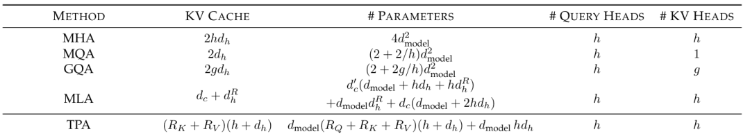
This reduces the per-token memory cost to (Table 2):

$(R_K + R_V) cdot (H + d_h)$

Compared to the standard cost of $2 cdot H cdot d_h$ , the compression ratio becomes:

$dfrac{(R_K + R_V)(H + d_h)}{2H d_h}$

For typical head dimensions (e.g., $d_h = 64$ or $128$ ) and small ranks (e.g., $R_K, R_V = 1$ or $2$ ), TPA achieves substantial KV cache reduction — often by an order of magnitude. This enables longer sequence inference under fixed memory budgets, making TPA especially attractive for deployment in resource-constrained environments.

**Table 2:** Comparison of different attention mechanisms along with TPA (source: Zhang et al., 2025).

PyTorch Implementation of Tensor Product Attention (TPA)

In this section, we will walk through the PyTorch implementation of the Tensor Product Attention. We’ll break down the code into the key components: the attention module, the transformer block, and the inference code.

Tensor Product Attention with KV Caching

We begin by implementing the core attention mechanism in the MultiHeadTPAAttention class. This class inherits from torch.nn.Module and sets up the necessary layers for the attention calculation.

import torch
import torch.nn as nn
import time
import matplotlib.pyplot as plt
import math

class MultiHeadTPAAttention(nn.Module):
    def __init__(self, d_model=128*128, num_heads=128, R_q=12, R_kv=4):
        super().__init__()
        self.d_model = d_model
        self.num_heads = num_heads
        self.R_q = R_q
        self.R_kv = R_kv
        self.head_dim = d_model // num_heads

        # Query projections
        self.Wq_a = nn.Linear(d_model, self.R_q*self.num_heads)
        self.Wq_b = nn.Linear(d_model, self.R_q*self.head_dim)

        # Key-value projections
        self.Wk_a = nn.Linear(d_model, self.R_kv*self.num_heads)
        self.Wk_b = nn.Linear(d_model, self.R_kv*self.head_dim)

        self.Wv_a = nn.Linear(d_model, self.R_kv*self.num_heads)
        self.Wv_b = nn.Linear(d_model, self.R_kv*self.head_dim)

        # Output projection
        self.Wo = nn.Linear(self.num_heads * self.head_dim, d_model)

    def forward(self, x, kv_cache):
        batch_size, seq_len, d_model = x.shape

        # Projections of input into latent spaces
        A_q, B_q = self.Wq_a(x), self.Wq_b(x)     # shape: (batch_size, seq_len, q_latent_dim)
        A_k, B_k = self.Wk_a(x), self.Wk_b(x)   # shape: (batch_size, seq_len, kv_latent_dim)
        A_v, B_v = self.Wv_a(x), self.Wv_b(x)   # shape: (batch_size, seq_len, kv_latent_dim)

        A_q = A_q.view(batch_size, seq_len, self.num_heads, self.R_q)
        B_q = B_q.view(batch_size, seq_len, self.R_q, self.head_dim)

        A_k = A_k.view(batch_size, seq_len, self.num_heads, self.R_kv)
        B_k = B_k.view(batch_size, seq_len, self.R_kv, self.head_dim)

        A_v = A_v.view(batch_size, seq_len, self.num_heads, self.R_kv)
        B_v = B_v.view(batch_size, seq_len, self.R_kv, self.head_dim)


        # Append to cache
        kv_cache['A_k'] = torch.cat([kv_cache['A_k'], A_k], dim=1)
        kv_cache['B_k'] = torch.cat([kv_cache['B_k'], B_k], dim=1)

        kv_cache['A_v'] = torch.cat([kv_cache['A_v'], A_v], dim=1)
        kv_cache['B_v'] = torch.cat([kv_cache['B_v'], B_v], dim=1)

        # Expand KV heads to match query heads
        A_k = kv_cache['A_k']
        B_k = kv_cache['B_k']

        A_v = kv_cache['A_v']
        B_v = kv_cache['B_v']

        Q = torch.matmul(A_q, B_q)
        K = torch.matmul(A_k, B_k)
        V = torch.matmul(A_v, B_v)

        # Attention score, shape: (batch_size, num_heads, seq_len, seq_len)
        scores = torch.matmul(Q.transpose(1, 2), K.transpose(1, 2).transpose(2, 3)) / math.sqrt(self.head_dim)
        # Attention computation
        attn_weight = torch.softmax(scores, dim=-1)

        # Compute attention output, shape: (batch_size, seq_len, num_heads, head_dim)
        output = torch.matmul(attn_weight, V.transpose(1,2)).transpose(1,2).contiguous()
        # Concatenate the heads, then apply output projection
        output = self.Wo(output.view(batch_size, seq_len, -1))

        return output, kv_cache

On Lines 1-5, we import the necessary PyTorch modules and other libraries for numerical operations and plotting. On Lines 7-28, we define the MultiHeadTPAAttention class, initializing parameters such as the model dimension (d_model), number of attention heads (num_heads), and the latent dimensions for queries (R_q) and keys/values (R_kv). We also define linear layers that project the input into query, key, and value components in the latent space, as well as an output projection layer.

On Lines 30-36, in the forward method, we take the input tensor x and the KV cache as arguments. We project the input x into latent representations A_q, B_q, A_k, B_k, A_v, and B_v using the defined linear layers. On Lines 34-45, we reshape these projected tensors to align with the multi-head attention structure.

On Lines 49-53, we append the newly computed key and value projections (A_k, B_k, A_v, B_v) to the existing KV cache. This is crucial for efficient autoregressive inference, as it avoids recomputing the keys and values for previous tokens. On Lines 56-64, we retrieve the updated key and value projections from the cache and then compute the Query (Q), Key (K), and Value (V) tensors by multiplying their respective A and B components.

On Lines 67-69, we calculate the attention scores by taking the dot product of the Query and Key tensors, scaled by the square root of the head dimension. We then apply the softmax function to obtain the attention weights. Finally, on Lines 72-76, we compute the attention output by multiplying the attention weights with the Value tensor, reshape the output, and apply the final output projection. The function returns the attention output and the updated KV cache.

Transformer Block

Next, we implement a simple Transformer block that incorporates the Tensor Product Attention module.

class TransformerBlock(nn.Module):
    def __init__(self,  d_model=128*128, num_heads=128, R_q=12, R_kv=4):
        super().__init__()
        self.attn = MultiHeadTPAAttention(d_model, num_heads, R_q, R_kv)
        self.norm1 = nn.LayerNorm(d_model)
        self.ff = nn.Sequential(
            nn.Linear(d_model, d_model * 4),
            nn.ReLU(),
            nn.Linear(d_model * 4, d_model)
        )
        self.norm2 = nn.LayerNorm(d_model)

    def forward(self, x, kv_cache):
        attn_out, kv_cache = self.attn(x, kv_cache)
        x = self.norm1(x + attn_out)
        ff_out = self.ff(x)
        x = self.norm2(x + ff_out)
        return x, kv_cache

On Lines 77-87, we define the TransformerBlock class, which includes an instance of our MultiHeadTPAAttention module, two instances of layer normalization (norm1 and norm2), and a feed-forward network (ff). The feed-forward network consists of two linear layers with a ReLU activation in between.

On Lines 89-94, in the forward method, the input x first passes through the attention layer along with the KV cache. The attention layer’s output is then added to the original input (a residual connection) and normalized. This is followed by the feed-forward network, and another residual connection and layer normalization. The function returns the output of the transformer block and the updated KV cache.

Inferencing Code

Next, we have the run_inference function, which simulates the autoregressive generation process.

def run_inference(block):
    d_model = block.attn.d_model
    num_heads = block.attn.num_heads
    kv_latent_dim = block.attn.R_kv

    seq_lengths = list(range(1, 50, 10))
    kv_cache_sizes = []
    inference_times = []

    kv_cache = {
        'A_k': torch.empty(1, 0, num_heads, kv_latent_dim),
        'B_k': torch.empty(1, 0, kv_latent_dim, d_model // num_heads),
        'B_v': torch.empty(1, 0, kv_latent_dim, d_model // num_heads),
        'A_v': torch.empty(1, 0, num_heads, kv_latent_dim),
    }

    for seq_len in seq_lengths:
        x = torch.randn(1, 1, d_model)  # One token at a time
        start = time.time()
        o, kv_cache = block(x, kv_cache)
        end = time.time()
        size = kv_cache['A_k'].numel() + kv_cache['B_v'].numel() + kv_cache['B_k'].numel() + kv_cache['A_v'].numel()
        kv_cache_sizes.append(size)
        inference_times.append(end - start)

    return seq_lengths, kv_cache_sizes, inference_times

The run_inference function (Lines 95-102) simulates the autoregressive generation process of a Transformer block. We initialize an empty KV cache (Lines 104-109) that stores the keys and values from previous tokens. We then iterate through a range of sequence lengths (Line 111), simulating the generation of one token at a time (Line 112). For each token, we pass it through the TransformerBlock (Line 114), which updates the KV cache. We measure the time taken for each step and the size of the KV cache (Lines 115 and 116).

After processing all the tokens for a given sequence length, we record the KV cache size and inference time. This process is repeated for different sequence lengths, allowing us to observe how the KV cache size and inference time change as the sequence grows. Finally, we return the collected data for plotting and analysis (Line 120).

Experimentation

plt.figure(figsize=(12, 5))
plt.subplot(1, 2, 1)

for latent_dim in [2, 4, 8, 16, 32]:
  mla_block = TransformerBlock(d_model=4096, num_heads=32, R_q=12, R_kv=latent_dim)
  seq_lengths, sizes, times = run_inference(mla_block)
  plt.plot(seq_lengths, sizes, label="TPA R_kv dim : {}".format(latent_dim))

plt.xlabel("Generated Tokens")
plt.ylabel("KV Cache Size")
plt.title("KV Cache Growth")
plt.legend()

plt.subplot(1, 2, 2)
for latent_dim in [2, 4, 8, 16, 32]:
    mla_block = TransformerBlock(d_model=4096, num_heads=32, R_q=12, R_kv=latent_dim)
    seq_lengths, sizes, times = run_inference(mla_block)
    plt.plot(seq_lengths, times, label="TPA R_kv dim : {}".format(latent_dim))


plt.xlabel("Generated Tokens")
plt.ylabel("Inference Time (s)")
plt.title("Inference Speed")

plt.legend()

plt.tight_layout()
plt.show()

Output:

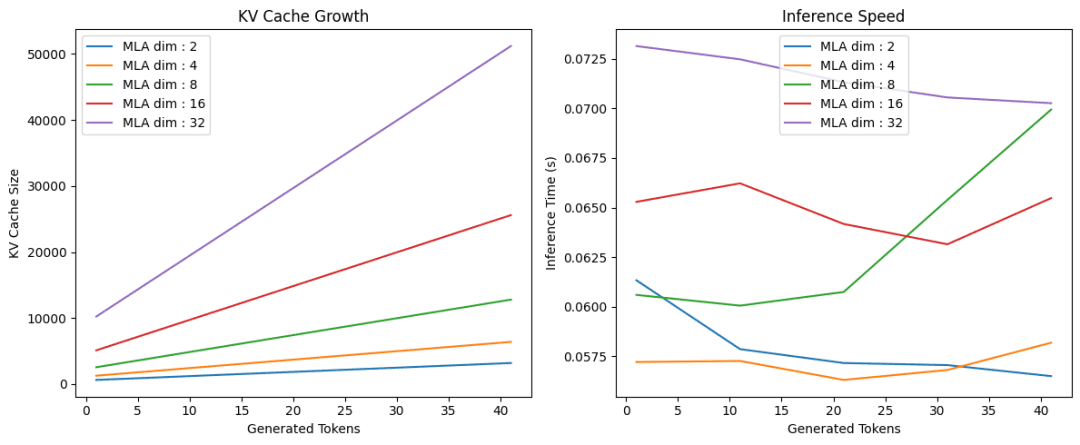
**Figure 2:** Reduction in KV Cache size by using Tensor Product attention of various latent dimensions (source: image by the author).

In this code (Lines 121-148), we conduct experiments to analyze the performance of the tensor product attention mechanism across different KV latent dimensions. We set up a figure with two subplots (Lines 121 and 122) to visualize the results. We then iterate through a list of different latent dimensions (Line 124). For each latent dimension, we create a TransformerBlock instance with the specified d_model, num_heads, R_q, and the current latent_dim for R_kv (Line 125). We then call the run_inference function (Line 126) with this block to get the sequence lengths, KV cache sizes, and inference times.

We then plot the KV cache sizes against the generated tokens (sequence lengths) on the first subplot (Lines 127-132) and the inference times against the generated tokens on the second subplot (Lines 138-143). This allows us to compare how different latent dimensions affect the KV cache growth and inference speed (Figure 2).

What’s next? We recommend PyImageSearch University.

Course information:
86+ total classes • 115+ hours hours of on-demand code walkthrough videos • Last updated: December 2025
★★★★★ 4.84 (128 Ratings) • 16,000+ Students Enrolled

I strongly believe that if you had the right teacher you could master computer vision and deep learning.

Do you think learning computer vision and deep learning has to be time-consuming, overwhelming, and complicated? Or has to involve complex mathematics and equations? Or requires a degree in computer science?

That’s not the case.

All you need to master computer vision and deep learning is for someone to explain things to you in simple, intuitive terms. And that’s exactly what I do. My mission is to change education and how complex Artificial Intelligence topics are taught.

If you’re serious about learning computer vision, your next stop should be PyImageSearch University, the most comprehensive computer vision, deep learning, and OpenCV course online today. Here you’ll learn how to successfully and confidently apply computer vision to your work, research, and projects. Join me in computer vision mastery.

Inside PyImageSearch University you’ll find:

&check; 86+ courses on essential computer vision, deep learning, and OpenCV topics
&check; 86 Certificates of Completion
&check; 115+ hours hours of on-demand video
&check; Brand new courses released regularly, ensuring you can keep up with state-of-the-art techniques
&check; Pre-configured Jupyter Notebooks in Google Colab
&check; Run all code examples in your web browser — works on Windows, macOS, and Linux (no dev environment configuration required!)
&check; Access to centralized code repos for all 540+ tutorials on PyImageSearch
&check; Easy one-click downloads for code, datasets, pre-trained models, etc.
&check; Access on mobile, laptop, desktop, etc.

Click here to join PyImageSearch University

Summary

In this third installment of our series on LLM Inference Optimization, we delve into Tensor Product Attention (TPA), a novel approach to reimagining attention representations. We explore how TPA leverages tensor decompositions to factorize queries, keys, and values into low-rank contextual components. This method significantly reduces KV cache size and seamlessly integrates with Rotary Positional Embeddings (RoPE), maintaining positional awareness without additional per-head parameters.

We examine the mechanics of TPA, contrasting it with the limitations of existing KV cache optimization strategies such as Grouped Query Attention (GQA) and Multi-Head Latent Attention (MLA). While GQA shares keys and values across query groups and MLA compresses KV representations into a shared latent space, TPA dynamically factorizes activations, storing KV states as compact sets of low-rank factors. This results in a memory cost that scales more efficiently with sequence length and head dimensionality.

Ultimately, we demonstrate how TPA paves the way for scalable, high-performance LLM inference by addressing the memory bottlenecks of traditional multi-head attention. By caching only the factorized components of keys and values, TPA offers a more memory-efficient solution for autoregressive decoding.

Citation Information

Mangla, P. “KV Cache Optimization via Tensor Product Attention,” PyImageSearch, P. Chugh, S. Huot, A. Sharma, and P. Thakur, eds., 2025, https://pyimg.co/6ludn

@incollection{Mangla_2025_kv-cache-optimization-via-tensor-product-attention,
  author = {Puneet Mangla},
  title = {{KV Cache Optimization via Tensor Product Attention}},
  booktitle = {PyImageSearch},
  editor = {Puneet Chugh and Susan Huot and Aditya Sharma and Piyush Thakur},
  year = {2025},
  url = {https://pyimg.co/6ludn},
}

To download the source code to this post (and be notified when future tutorials are published here on PyImageSearch), simply enter your email address in the form below!

Download the Source Code and FREE 17-page Resource Guide

Enter your email address below to get a .zip of the code and a FREE 17-page Resource Guide on Computer Vision, OpenCV, and Deep Learning. Inside you’ll find my hand-picked tutorials, books, courses, and libraries to help you master CV and DL!

The post KV Cache Optimization via Tensor Product Attention appeared first on PyImageSearch.

Like 0

Liked Liked